Deconstructing Economic Equilibrium: Insights into Ex Ante Aggregate Demand and Autonomous Expenditure

In an economy without a government, the ex ante aggregate demand for final goods is the sum total of the ex ante consumption expenditure and ex ante investment expenditure on such goods, viz. AD = C + I. 

• Substituting the values of C and I, aggregate demand for final goods can be written as

AD =  C + I  + c.Y

• If the final goods market is in equilibrium this can be written as

Y =  C + I + c.Y

• where Y is the ex ante, or planned, output of final goods. 
• This equation can be further simplified by adding up the two autonomous terms, C and I , making it

Y = A + c.Y

• where A = C + I is the total autonomous expenditure in the economy.
• In practice, these two elements of autonomous expenditure exhibit distinct behaviors.
• C, representing the subsistence consumption level of an economy, remains relatively stable over time.

Uncovering Discrepancies Between Ex Ante Supply and Demand in Final Goods Market

In the context of economic equilibrium, the two sector model plays a pivotal role in understanding the dynamics between ex ante supply and demand.

• Conversely, I has been observed to undergo periodic fluctuations.
• It’s important to note that Y on the left side of the equation signifies the ex ante output or the planned supply of final goods. 
• Conversely, the expression on the right side represents the ex ante or planned aggregate demand for final goods in the economy. 
• These two values are equal only when the final goods market, and consequently the entire economy, is in equilibrium.
• If the ex ante demand for final goods falls short of the planned output of final goods for a given year will not hold. 
• In such cases, unintended accumulation of inventories occurs.

The Nuances of Planned and Unplanned Inventory Investment in Economic Equations

Investment: It should be noted that inventories or stocks refers to that part of output produced which is not sold and therefore remains with the firm.

Inventory Investment: It is known as unanticipated accumulation or depletion of inventories.

• It can be either positive (a rise in inventory) or negative (a reduction in inventory). 
• Inventory investment can occur for two reasons:
  • Planned inventory investment: Firms decide to maintain some stocks for various purposes or
  •  Unplanned inventory investment: actual sales differ from the planned sales, forcing firms to either increase or reduce existing inventories.
• Therefore, even if planned Y exceeds planned C + I, actual Y will equal actual C + I, with the additional output appearing as unintended accumulation of inventories in the ex post I on the right hand side of the accounting identity.

Government’s Fiscal Footprint: Shaping Economic Equilibrium in the Two Sector Model

In the two sector model, the economic landscape expands with the introduction of the government’s pivotal role.

• The primary fiscal variables that influence aggregate demand for final goods and services are fiscal variables Tax (T) and Government Expenditure (G). 
• Government, through its spending G on final goods and services, contributes to aggregate demand similar to households. 
• Conversely, taxes levied by the government subtract a portion of income from households, resulting in disposable income becoming Yd = Y – T.
• Households only allocate a fraction of this disposable income to consumption purposes. 
• Hence the equation has to be modified in the following way to incorporate the government:

Y = C + I + G + c (Y – T)

A Two-Stage Approach to Short-Run Macroeconomic Analysis with Fixed Price Levels

In microeconomic theory, Analyzing the equilibrium of supply and demand in a single market, the interaction of the demand and supply curves simultaneously determines both the equilibrium price and the equilibrium quantity. 

However, in macroeconomic theory, we approach the analysis in two stages:

• • First stage: In this, calculating macroeconomic equilibrium while treating the price level as fixed.

• Second stage: In this, price levels allow to vary and then analyze macroeconomic equilibrium under these conditions.

The justification for taking the price level as fixed initially can be explained for two reasons:

• In the first stage, assume an economy with unused resources like machinery, buildings, and labor. 
  • In such a situation, the law of diminishing returns does not apply.
  • This means that additional output can be produced without an increase in marginal cost. 
  • Therefore, the price level remains stable even if the quantity produced changes.
• This assumption of a fixed price level is primarily a simplifying assumption made at the early stages of macroeconomic analysis, which can be considered in later stages of analysis.

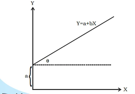
Intercept form of the linear equation

Macroeconomic Equilibrium: Analyzing Consumer Demand and Linear Relations with Fixed Price Levels

(A) Graphical Method

• As already explained, the consumer’s demand can be expressed by the equation

C= C  +cY

• Where C is  Autonomous expenditure and 
• c is the marginal propensity to consume
• The intercept form of a linear equation is a way to represent a straight line on a graph. It’s written in the form

Y = a + bX

• Here, the variables are X and Y and there is a linear relation between them. 
• a and b are constants. 
• This equation is depicted in the figure. The constant ‘a’ is shown as the “intercept” on the Y axis, i.e, the value of Y when X is zero. The constant ‘b’ is the slope of the line i.e. tangent = b.

Consumption Function – Graphical Representation 

• Using the same logic, the consumption function can be shown as follows (Refer Figure):

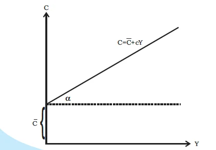
Consumption function with intercept C

• Consumption function C= C  +cY 
• Where,
  • C = intercept of the consumption function, 
  • c = slope of consumption function = tan

Investment Function – Graphical Representation 

• In a two sector model, there are two sources of final demand, 
  • The first is consumption and 
  • The second is investment. 
• The investment function was shown as I = I
• Graphically, this is shown as a horizontal line at a height equal to I  above the horizontal axis(Refer Figure).

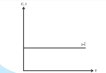
Investment function with I as autonomous

• In this model, I is autonomous which means, it is the same no matter whatever is the level of income.

Aggregate Demand: Graphical Representation

• The Aggregate Demand function represents the combined demand for goods and services in an economy, consisting of both consumption and investment. 

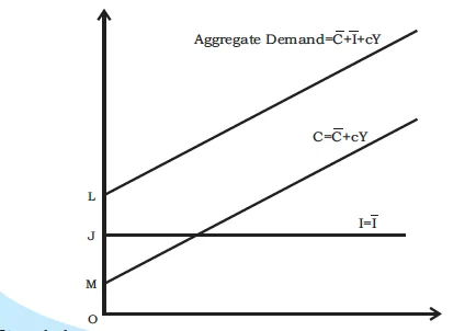
Aggregate demand is obtained by vertically adding the consumption and investment functions.

• Graphically, this can be visualized by vertically adding the consumption and investment functions to derive the Aggregate Demand curve.
• Here,  
  • OM =  C
  • OJ = I 
  • OL = C + I 
• The aggregate demand function is parallel to the consumption function i.e., they have the same slope c. 
• It may be noted that this function shows ex ante demand(Refer Figure)

Fixed Price Levels and the 45-Degree Line Representation of Supply Dynamics

• In microeconomic theory, a typical graph representing the supply curve displays quantity supplied on the horizontal axis and price on the vertical axis.
• However, in the initial stages of macroeconomic analysis, we consider the price level to be fixed.
• In this context, we assume that the aggregate supply, or the Gross Domestic Product (GDP), can smoothly vary up or down because there are unused resources of various types available. 
• Regardless of the level of GDP, it is assumed that the economy will supply exactly that amount, and the price level is not a determining factor in this scenario. 
• This type of supply situation is represented by a 45-degree line on the graph (Refer Figure).

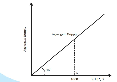
Aggregate supply curve with 45-degree line.

• The distinctive feature of the 45-degree line is that every point on it has identical horizontal and vertical coordinates.

Equilibrium: Unifying Ex Ante Demand and Supply through Graphical and Algebraic Insights

 In the two sector model, achieving equilibrium becomes a complex yet essential task. 

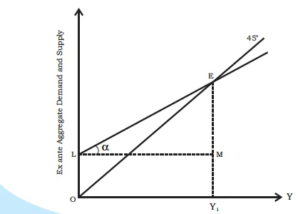
• Equilibrium is depicted by combining ex ante aggregate demand and supply on a diagram (as shown in Figure). 

Equilibrium of ex ante aggregate demand and supply

• The point at which ex ante aggregate demand equals ex ante aggregate supply represents the equilibrium. 
• In this context, the equilibrium point is denoted as E, and the corresponding equilibrium income level is ‘OY1.

(B) Algebraic Method

• Ex ante aggregate demand = I  + C + cY
• Ex ante aggregate supply = Y
• Equilibrium requires that the plans of suppliers are matched by plans of those who provide final demands in the economy. 
• Thus, in this situation, ex ante aggregate demand = ex ante aggregate supply(Refer Figure),

C + I  + cY = Y

Y (1-c) = C + I 

Y = ( C + I ) / (1-c)

Ripple Effects of Autonomous Demand Changes: the Multiplier Impact on Income and Output in Macroeconomic Equilibrium

• The equilibrium level of income is contingent on aggregate demand, and alterations in aggregate demand can result from various factors.
• Changes in aggregate demand can arise from:
  • Change in consumption: This can occur due to two factors, change in C and changes in c.
  • Change in investment: While  assuming that investment is autonomous and not influenced by income, it simply means that it’s not directly tied to income. 
• There are several variables, apart from income, that can affect investment. 
  • Notably, the availability of credit plays a significant role; when credit is easily accessible, it tends to stimulate investment. 
  • Another critical factor is the interest rate; it represents the cost of acquiring investible funds, and when interest rates are high, firms often reduce their level of investment.

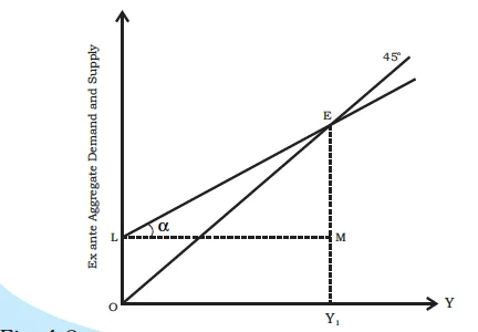
Equilibrium of ex ante aggregate demand and supply

• In the new equilibrium, output and aggregate demand have increased by an amount E1G = E2G, which is greater than the initial increment in autonomous expenditure, 

I  =  E1F = E2J. 

• Thus an initial increment in the autonomous expenditure seems to have a multiplier on the equilibrium values of aggregate demand and output.

Demystifying the Investment Multiplier Mechanism and its Impact on Total Output

• Exploring the multiplier mechanism within the context of a two sector model provides valuable insights into the dynamics of economic growth. In the two sector model, where the economy is divided into consumption and investment sectors, the effects of an autonomous change in aggregate demand are profound. 
• The change in equilibrium income by 50 units (from 250 to 300) due to a change in autonomous expenditure of 10 units can be understood through the multiplier mechanism, which is explained as follows:
  • The production of final goods involves various factors such as labor, capital, land, and entrepreneurship. 
  • Assuming no indirect taxes or subsidies, the total value of final goods output is distributed among these factors as payments – wages for labor, interest for capital, rent for land, and the remainder as profit to entrepreneurs.
  • The sum of these aggregate factor payments in the economy, known as National Income, is equal to the aggregate value of the final goods output, which is the Gross Domestic Product (GDP).
  • The increase in the equilibrium value of total output is greater than the initial increase in autonomous expenditure.
• Investment Multiplier: The ratio of the total increase in the equilibrium value of final goods output to the initial increase in autonomous expenditure is known as the investment multiplier of the economy. 
• The ratio of the total increase in the equilibrium value of final goods output to the initial increase in autonomous expenditure is known as the investment multiplier of the economy. 
• Recalling that 10 and 0.8 represent the values of I = A and mpc, respectively, 
• The expression for the multiplier can be explained as

Investment Multiplier  = Y / A 

= 1 / (1-c)

= 1 / S

• Where: ΔY is the total increase in final goods output and c = mpc. 

• It is important to note that the size of the multiplier is influenced by the value of c. 
  • When c becomes larger, the multiplier increases as well.
•  In other words, a higher marginal propensity to consume results in a more significant multiplier effect.

DOWNLOAD PDF