Introduction: Diminishing Marginal Product & Variable Proportions

The Law of Diminishing Marginal Product and the Law of Variable Proportions are fundamental principles in economics and production. The Law of Diminishing Marginal Product states that as additional units of a variable input are added to a fixed quantity of other inputs, the marginal product of that variable input will eventually decrease. The Law of Variable Proportions further explores how changes in the combination of inputs can affect production output and efficiency.

Law of Diminishing Marginal Product: Increase, Peak, and Decline

• Law: It states that the tendency of the marginal product (MP) to first increase and then fall is called the law of diminishing marginal product.
  • Increasing the employment of an input, with other inputs fixed, eventually a point will be reached after which the resulting addition to output (i.e., marginal product of that input) will start falling.

Law of Variable Proportions: Marginal Product Rise and Decline

• Law: It states that  the marginal product of a factor input initially rises with its employment level. But after reaching a certain level of employment, it starts falling.

• Reason:

• • As we hold one factor fixed and keep increasing the other, the factor proportions change. 

• • Initially, increasing the amount of the variable input, the factor proportions become more and more suitable for the production and marginal product increases. 

• • However, after a certain level of employment, the production process becomes too crowded with the variable input.

Shapes of Total Product, Marginal Product and Average Product Curves: Curves of Production Output

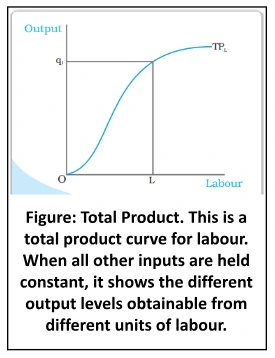
• An increase in the amount of one of the inputs keeping all other inputs constant results in an increase in output. 
• The Total Product Curve: In the input-output plane is a positively sloped curve. 
  • Refer to Figure which shows the shape of the total product curve for a typical firm. 
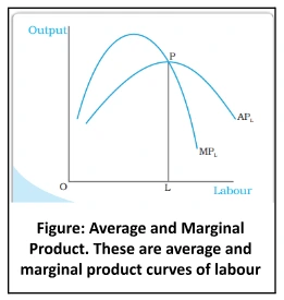
• Law of Variable Proportions: According to it, the marginal product of an input initially rises and then after a certain level of employment, it starts falling.
• Inverse ‘U’-Shaped: The MP curve, therefore, looks like an inverse ‘U’-shaped curve as in Figure.
• The Relationship Between Marginal Product (MP) and Average Product (AP): As we increase the amount of input, the MP rises. 
  • AP being the average of marginal products, also rises but rises less than MP. 
  • After a point, the MP starts falling.
  • However, as long as the value of MP remains higher than the value of the AP, the AP continues to rise. 
  • Once MP has fallen sufficiently, its value becomes less than the AP and the AP also starts falling. So the AP curve is also inverse ‘U’-shaped. 

Returns to Scale: Constant, Increasing, and Decreasing Returns

• The law of variable proportions arises because factor proportions change as long as one factor is held constant and the other is increased.
• One special case in the long run occurs when both factors are increased by the same proportion, or factors are scaled up.
•  There are three types of scale 
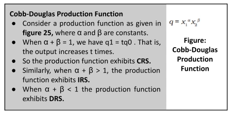
  • Constant returns to scale (CRS): When a proportional increase in all inputs results in an increase in output by the same proportion, the production function is said to display Constant returns to scale (CRS). 
  • Increasing Returns to Scale (IRS): When a proportional increase in all inputs results in an increase in output by a larger proportion, the production function is said to display Increasing Returns to Scale (IRS).
  • Decreasing Returns to Scale (DRS): It holds when a proportional increase in all inputs results in an increase in output by a smaller proportion.
• Example: Suppose in a production process, all inputs get doubled. 
  • If the output gets doubled, the production function exhibits CRS.
  • If output is less than doubled, the DRS holds, and 
  • If it is more than doubled, the IRS holds.

Costs: Strategies for Least Cost Production

• Input Combinations for Least Cost Production: In order to produce output, the firm needs to employ inputs. 
  • However a given level of output, typically, can be produced in many ways.
  • For every level of output, a firm chooses the least cost input combination. 
• Thus the cost function describes the least cost of producing each level of output given the prices of factors of production and technology. 

Short Run Costs: Fixed and Variable Factors

• Fixed Factors of Production: In the short run, some of the factors of production cannot be varied, and therefore, remain fixed.
• Total Fixed cost (TFC): It is the cost that a firm incurs to employ these fixed inputs.
  • Whatever amount of output the firm produces, this cost remains fixed for the firm. 
• To produce any required level of output, the firm, in the short run, can adjust only variable inputs. 
• Total Variable Cost (TVC): The cost that a firm incurs to employ these variable inputs is called the total variable cost (TVC). 
• Total Cost (TC): Adding the fixed and the variable costs, we get the total cost (TC) of a firm i.e., TC = TVC + TFC.
• Short-Run Average Cost (SAC): It is incurred by the firm. It  is defined as the total cost per unit of output. We calculate it as SAC = TC/q.
• Average Variable Cost (AVC): It is defined as the total variable cost per unit of output. We calculate it as AVC = TVC/q.
• Also, the average fixed cost (AFC) is AFC = TFC/q. So, clearly SAC = AVC + AFC.

Long Run Costs: Variable Inputs and Total Cost Analysis

• Variable Inputs: In the long run, all inputs are variable. There are no fixed costs. The total cost and the total variable cost, therefore, coincide in the long run. 
• Long-Run Average Cost (LRAC): It is defined as cost per unit of output, i.e. LRAC = TC/q.
• Long-Run Marginal Cost (LRMC): It is the change in total cost per unit of change in output.
• Just like the short run, in the long run, the sum of all marginal costs up to some output level gives us the total cost at that level.

Conclusion

In this chapter, we have discussed the problem of variable inputs, output and cost associated with a product in a firm. For different combinations of inputs, the production function shows the maximum quantity of output that can be produced. In the short run, some inputs cannot be varied and in the long run, all inputs can be varied. In order to produce output, the firm chooses least cost input combinations. 

DOWNLOAD PDF