Connecting Marginal Costs to Supply: Dynamics of a Market supply Curve

A firm’s supply curve is fundamentally linked to its marginal cost curve, implying that factors affecting the marginal cost curve will, in turn, influence the supply curve.

Innovative Efficiency: Impact on Costs and Market Supply Curve

Technological Progress:  Boosting Output and Cutting Costs

• A firm utilises two factors of production – capital and labour, to produce a specific good.
• Organizational Innovation: It is introduced, leading to enhanced productivity where the same levels of capital and labor now yield more units of output.
• Innovation’s Impact on Input Efficiency: This innovation allows the firm to use fewer units of input to produce the same level of output.
• Efficiency Boost: Tech’s Effect on Marginal Costs
  • Improving Production Efficiency: The technological advancement is expected to reduce the firm’s marginal cost at any given level of output.
  • This is represented by a rightward (or downward) shift of the Marginal Cost (MC) curve.
• Effect on Supply Curve: Rightward Shift Impact
  • A Rightward Shift: Since the supply curve is a segment of the MC curve, technological progress translates to a rightward shift in the supply curve.
  • Increased Output Supply: Consequently, at any given market price, the firm is now able to supply more units of output.

Input Price Impact: Rising Costs and Marginal Effects

• The supply curve of a firm is directly influenced by the prices of inputs used in production.
• Rising Input Prices: Effect on Production Costs
  • Increase in Cost of Production: An increase in the price of an input, such as the wage rate of labour, leads to a rise in the cost of production.
  • Increase Average and Marginal Costs: This rise in production cost subsequently results in an increase in both the firm’s average cost and marginal cost at any given level of output.
• Shift in Marginal Cost (MC) Curve: Illustrating Marginal Cost Increase
  • The increase in marginal cost is graphically represented by a leftward (or upward) shift of the MC curve.
• Market Supply Curve Shift: Consequent of Marginal Cost Changes
• • Due to the shift in the MC curve, the firm’s supply curve also shifts to the left.
  • This shift implies that at any given market price, the firm is now able to supply fewer units of output.

Unit Tax Effects: Long-Run Costs and Supply Shift

• Definition: A unit tax is a tax that the government imposes per unit sale of output.
• Example: A unit tax of Rs 2 means a firm selling 10 units will pay a total tax of Rs 20 to the government.
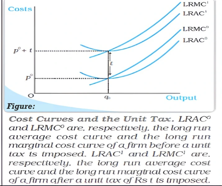
• Tax Impact: Effect on Costs Shifts LRMC and LRAC Upward
  • Before the Imposition of a Unit Tax:, the firm operates at Long Run Marginal Cost (LRMC0) and Long Run Average Cost (LRAC0). 
  • Post Imposition of a Unit Tax: After tax of Rs t, both the long-run average cost and long-run marginal cost increase by Rs t per unit of output, transitioning to LRMC1 and LRAC1 respectively.
• Unit Tax Effects: Long-Run Supply Curve Shift and Output Impact
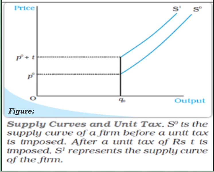
  • Determining the Long-Run Supply Curve: The long-run supply curve of a firm is derived from the rising part of the LRMC curve from and above the minimum LRAC, along with zero output for all prices below the minimum LRAC.
  • Upon Imposition of the Unit Tax: The long-run supply curve shifts to the left, represented by the transition from S0 to S1 .
  • Impact of Unit Tax on Firm’s Output: This shift implies that at any given market price, the firm now supplies fewer units of output due to the unit tax.
  • Tax’s Impact on a Firm’s Long-Run: The graphical representation in Figures  elucidates the upward shift in cost curves and the leftward shift in the supply curve post-unit tax imposition, highlighting the tax’s impact on a firm’s long-run cost structure and supply behaviour.

Market Supply Curve: Aggregating Firm Outputs at Varying Prices

The market supply curve illustrates the aggregate output levels produced by firms in a market against different values of market price, with output levels on the x-axis and market prices on the y-axis.

Building Market Supply Curve: Combining Firms’ Outputs at Price Tiers

• Aggregate Output: In a market with n firms, the aggregate output at a fixed market price p is the sum of the supplies of individual firms at that price.
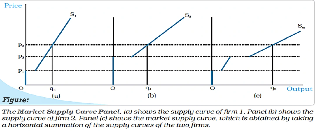
• Constructing the Market Supply Curve: Geometric construction of the market supply curve can be illustrated with two firms having different cost structures.
  • Firm 1 and Firm 2 have different threshold prices below which they will not produce, denoted as p1​ and p2​ respectively, with 2>p2​>p1​. As shown in Figure .
  • Panels (a) and (b) show the supply curves of Firm 1 (S1​) and Firm 2 (S2​) respectively.
  • Panel (c) illustrates the market supply curve (Sm​) derived by horizontally summing the supply curves of the two firms.
• Market Supply Behavior at Different Price Thresholds:
• • When Market Price is Below p1​:  Neither firm produces, hence the market supply is zero.
  • Between Prices p1​ and p2​: Only Firm 1 produces, making the market supply curve coincide with S1​.
  • At Prices Equal to or Above p2​: Both firms produce, and the market supply is the sum of their individual supplies.

Dynamic Market Supply Curve: Responding to Changes in Firm Numbers

• Fixed Number of Firms: The market supply curve is derived assuming a fixed number of firms.
• Changes in the Number of Firms: It shifts the market supply curve.
  • An increase in firms shifts it to the right, 
  • While a decrease in firm shifts it to the left.
• A numerical example is mentioned to supplement the graphical analysis;
  • Notice that S1(p) indicates that (1) firm 1 produces an output of 0 if the market price, p, is strictly less than 10, 
  • And (2) Firm 1 produces an output of (p – 10) if the market price, p, is greater than or equal to 10.

• Let the supply curve of firm 2 be as follows:
  • The interpretation of S2(p) is identical to that of S1(p), and is, hence, omitted.
  • Now, the market supply curve, Sm(p), simply sums up the supply curves of the two firms; in other words

• But, this means that Sm(p) is as follows

DOWNLOAD PDF